Global Oil Reserves vs Consumption: Power BI Deneb Template
Create a stunning dual-axis timeline visual in Power BI using Deneb and Vega. Compare 25 years of global oil reserves against consumption with interactive annotations.
This template creates a dual-axis timeline visual in Power BI using Deneb and the Vega grammar. It compares 25 years of global proven oil reserves against global consumption, with annotation lines for the two events that distort the series more than anything else: the 2003 Venezuela heavy-oil reclassification and the 2020 demand collapse.
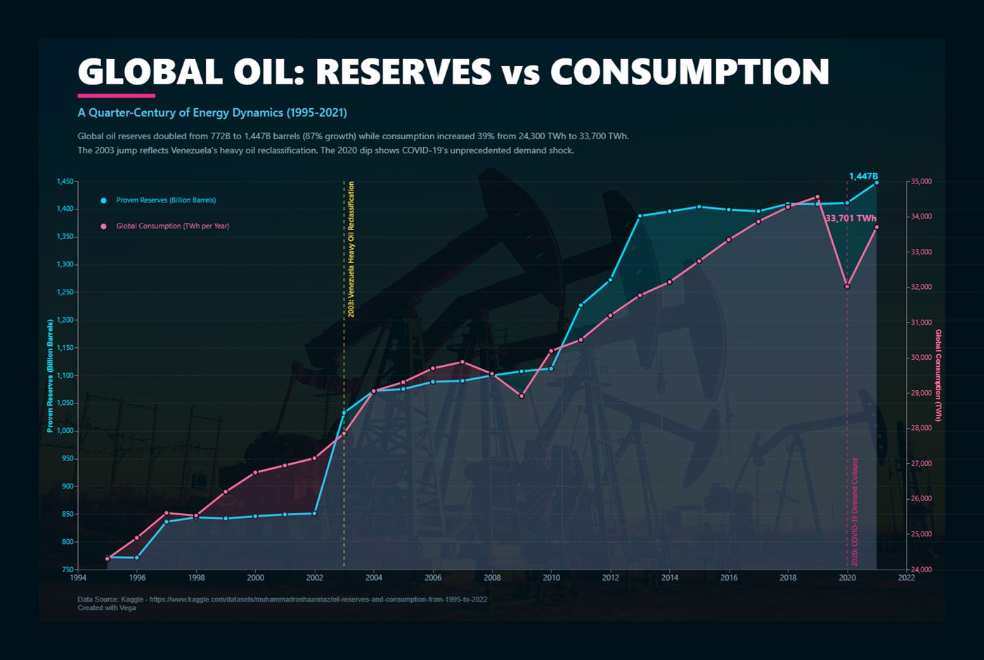
Dual-axis timeline comparing proven oil reserves with global consumption (1995-2021)
When a dual axis is the right choice
Two y-axes are usually a warning sign. They are defensible here for one reason: reserves (a stock, measured in billion barrels) and consumption (a flow, measured in TWh) are different quantities in different units, and the point of the chart is the divergence in their shapes, not a comparison of their magnitudes.
Use it when all three are true:
- The two series are genuinely different units, so a single axis would be meaningless.
- The reader's question is about direction and turning points, not about which line is bigger.
- Both axes start at zero, or you clearly label that they do not.
If your two series share a unit, do not use this template — index both to 100 at the first year and plot them on one axis instead. Anything else invites the reader to compare line heights that carry no meaning.
The data you need
The visual expects one row per year with three columns. Nothing else is required, and the spec projects away everything it does not use.
| Column | Type | Example | Notes |
|---|---|---|---|
| year | Whole number | 2019 | Not a date. A date column adds a hierarchy Deneb then has to flatten. |
| total\_reserves | Decimal | 1732.4 | Billion barrels, end of year. |
| total\_consumption | Decimal | 33700 | TWh, full year. |
The sample values baked into the template come from the BP Statistical Review of World Energy series (now published by the Energy Institute), aggregated to world totals. Swap in your own figures before publishing anything — the numbers here are illustrative and stop at 2021.
Complete Vega specification
Download the full JSON and paste it straight into the Deneb editor:
Adding it to a report
- Install Deneb: Visualizations pane, three dots, Get more visuals, search Deneb, Add.
- Drop the visual on the canvas and drag
year,total_reservesandtotal_consumptioninto the Values well. - Open the editor with the pencil icon, choose Vega (not Vega-Lite) as the provider.
- Paste the JSON over the starter spec and click Apply.
- Set the canvas size to roughly 1400 x 900 so the fixed padding and annotation offsets land where they were designed to.
Mapping your own field names
Rather than renaming columns in your model, rename them inside the projection transform. This keeps the rest of the spec untouched:
  "data": [
    {
      "name": "world_data",
      "values": {{ values | asJSON }},
      "transform": [
        {
          "type": "project",
          "fields": [
            {"field": "YourYearField", "as": "year"},
            {"field": "YourReservesField", "as": "total_reserves"},
            {"field": "YourConsumptionField", "as": "total_consumption"}
          ]
        }
      ]
    }
  ]
The {{ values | asJSON }} token is Deneb's dataset placeholder. Leave it exactly as written — it is replaced at render time with the rows Power BI passes in.
How the two scales are wired
Each series gets its own linear scale over its own field, and each scale is bound to a different side of the plot. The nice flag is what keeps the gridlines on round numbers:
  "scales": [
    {
      "name": "xscale", "type": "point",
      "domain": {"data": "world_data", "field": "year"},
      "range": [0, {"signal": "chartWidth"}], "padding": 0.02
    },
    {
      "name": "yReserves", "type": "linear", "nice": true, "zero": true,
      "domain": {"data": "world_data", "field": "total_reserves"},
      "range": [{"signal": "chartHeight"}, 0]
    },
    {
      "name": "yConsumption", "type": "linear", "nice": true, "zero": true,
      "domain": {"data": "world_data", "field": "total_consumption"},
      "range": [{"signal": "chartHeight"}, 0]
    }
  ]
Both scales include "zero": true deliberately. Letting either axis float to its data minimum would exaggerate the 2020 dip into something that looks like a collapse of supply rather than a 7% fall in demand.
The annotation layer
Annotations are what turn this from a chart into an explanation. Each one is a dashed rule plus an angled label, driven by a small inline dataset so you can add or remove events without touching the marks:
  {
    "name": "events",
    "values": [
      {"year": 2003, "label": "Venezuela heavy oil reclassified", "colour": "#FFD93D"},
      {"year": 2020, "label": "COVID-19 demand collapse", "colour": "#F72585"}
    ]
  }
Keep it to two or three. Every extra line costs the reader attention, and an annotated chart with six callouts reads as noise. If you need more, the events belong in a table underneath the visual.
Customising the look
- Colours:
#00D9FFreserves,#FF6B9Dconsumption,#001219background,#FFD93Dand#F72585for the two annotations. - Axis titles: "Proven Reserves (Billion Barrels)" and "Global Consumption (TWh)" — always name the unit on a dual-axis chart.
- Font: the
fontMainsignal sets it once for every text mark. - Area opacity: keep the fills below about 0.25 or the overlap turns muddy where the series cross.
Troubleshooting
- Blank visual, no error: the projection is renaming a field that does not exist. Field names in the transform are case-sensitive and must match the Power BI column name exactly.
- Both lines sit flat at the bottom: your measure is returning text. Cast it to a decimal in the model, not in the spec.
- Only one year shows: Power BI is aggregating. Put
yearin the Values well as "Don't summarize". - Annotations land off-centre: they are positioned by the same
xscale, so an annotation year that is missing from the data has nowhere to sit. Add the year with null measures. - Labels clipped at the edges: raise the top-level
padding; Deneb does not expand the canvas for overflowing text.
Performance and accessibility
Twenty-five rows render instantly, but Vega re-evaluates the whole spec on every cross-filter. If this visual sits on a page with heavy slicers, exclude it from interaction via Format, Edit interactions. On the dark background, the cyan and pink both clear WCAG AA against #001219; if you re-theme to a light background, they will not — re-test the pairs before shipping.
What the sample data actually shows
- Proven reserves rose from 772B to 1,447B barrels, roughly 87%, most of it in two discrete reclassification steps rather than gradual discovery.
- Consumption grew 39%, from about 24,300 TWh to 33,700 TWh, on a far smoother path.
- The 2003 step is an accounting change, not a discovery — worth annotating precisely because a reader will otherwise misread it.
- 2020 is the only year in the series where consumption falls sharply, about 7.4%.
Where to go next
Enable Deneb's tooltip handling to expose exact values on hover, and add a selection signal if you want the timeline to cross-filter the rest of the page. For a different take on comparing two periods, the revenue variance slope chart does it in pure DAX and SVG with no custom visual at all. If you want this built against your own data, get in touch.